Help Page
Index
- Introduction
- Available Methods
- Corrected Mutual Information
- Correction for low number of sequences
- Sequence clustering
- Correction for conservation or entropy of each residue
- Z-socres transformation
- Mean-field Direct Coupling Analysis (EVfold-mfDCA)
- PSICOV Precise strutural contact prediction using sparse inverse covariance matrix
- Sequence retrieval and MSA construction
- Sequence retrieval
- Multiple Sequence alignment
- Multiprotein alignment construction
- Upload your own alignments
- Inputs for running a job
- Server Results
- References
Introduction
This server allows users to analyse coevolutionary relationships between groups of proteins with three state of the art coevolutionary algorithms: corrected Mutual Information (1), DCA (2) and PSICOV (3). Also offer a comparative visualization of the results, allowing the comparison between methods and the election of which method suits better to solve a particular biological question.
Available Methods
Corrected Mutual Information score
Mutual information (MI) theory is often applied to predict positional correlations in a multiple sequence alignment (MSA) to make possible the analysis of those positions structurally or functionally important in a given fold or protein family.
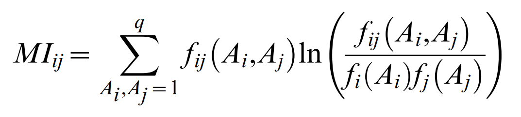
The MI between two positions in an MSA is given by the relationship:
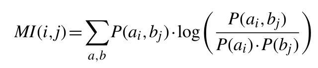
where P(ai, bi) is the frequency of amino acid a occurring at position i and amino acid b occurring at position j in the same sequence, P(ai) is the frequency of amino acid a at position i and P(bj) is the frequency of amino acid b at position j.
We use a transformed MI score as described in [1] with correction for low number of sequences (low count correction), sequence redundancy (sequence clustering), for lowering the background signal imposed by phylogeny and noise (average product correction) and a sequence-based Z-score permutation.
Correction for low number of sequences
The amino acid frequencies, P(a, b), are normalized from N(a,b), the number of times an amino acid pair (a, b) is observed at positions i and j in the MSA. From N(ai, bi), P(ai, bj) is calculated as (λ + N(ai, bi))/N, where:

It is clear that for MSAs of limited size, a large fraction of the P(ax, by) values will be estimated from a very low number of observations, and their contribution to MI could be highly noisy. To deal with such low counts, the parameter λ was introduced. The initial value for the variable N(ai, bj) = λ is set for all amino acid pairs. Only for MSAs with a small number of sequences, where a large fraction of amino acid pairs remain unobserved, will λ influence the amino acids occupancy calculation. For large MSAs, most amino acid pairs will be observed at least once, and the influence of λ will be minor.
We investigated how the performance depended on the values used for λ on a small independent dataset. The maximal performance was achieved for a value of λ equal to 0.05, but similar results are obtained in the range 0.025-0.075. This value was consistently found to be optimal for all datasets independently of size, evolutionary model, or rate of evolution [1].
Sequence clustering
When dealing with biological data, MSAs will often suffer from a high degree of unnatural sequence redundancy. It is hence expected that the sequence clustering would improve the accuracy of the MI calculation. We employed a Hobohm 1 algorithm to define sequence clusters, and assign each sequence within a given cluster a weight corresponding to one divided by the number of sequences in the cluster. Clusters were defined at a sequence identity threshold of 62%. The performance remains stable for threshold values in the range 40-75%. When accumulating the amino acid concurrencies, the sequence weight, rather that the value one, was used.
Correction for conservation or entropy of each residue
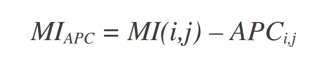
The MI value between two residues depends strongly on the conservation or entropy of the two residues. We apply the Average Product Corection (APC), proposed by Dunn et al. (2008), that defines an APC, and subtracts this value from MI:
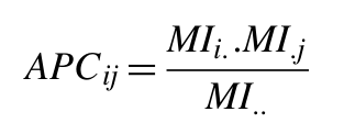
where MIi -as before- is the average MI value of residue i to all other residues in the MSA, and MI.. is the average MI value over all pairs of residues in the MSA.
Z-scores transformation
In a Z-score transformation, all prediction scores are compared with a distribution of prediction scores obtained from a large set of randomized MSAs. The Z-score is then calculated as the number of standard deviations that the observed MI value falls above the mean value obtained from the randomized MSAs. We applied a sequence-based Z-score procedure for MSA permutation that tests the hypothesis that the sequences are not homologous. The permutations were made with gaps fixed in their original positions and boundaries. The background mean and SD values were estimated from 100 such randomizations. It should be noted that sequence-based Z-score does not test for the appropriated null hypothesis (the columns not being correlated), and that sequence-based Z-score hence should be interpreted only as an additional prediction score [1].
Mean-field Direct Coupling Analysis (EVfold-mfDCA)
Note: this server uses FreeContact, an open-source EVfold-mfDCA implementation [4].
Computation of DCA residue pair coupling parameters in the maximum entropy model as described in [2]
To compute the effective pair couplings and single residue terms in the maximum entropy model two conditions must be satisfied. The first condition is maximal agreement between the expectation values of pair frequencies (marginals) from the probability model with the actually observed frequencies:
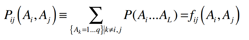
Where Ai and Aj are particular amino acids sequence positions i and j. The second condition is maximum entropy of the global probability distribution, which ensures a maximally evenly distributed probability model and can be satisfied without violating the first condition:
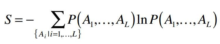
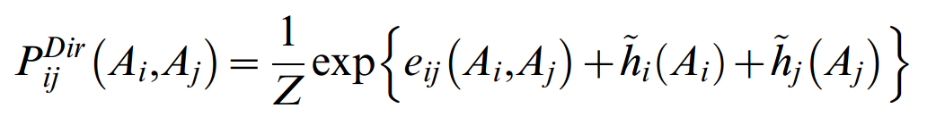
The solution of the constrained optimization problem defined by these conditions, using the formalism of Lagrange multipliers, is of the form:
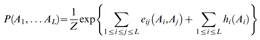
This global statistical model is formally similar to the statistical physics expression for the probability of the configuration of a multiple particle system, which is approximated in terms of a Hamiltonian that is a sum of pair interaction energies and single particle couplings to an external field. In this analogy, a sequence position i corresponds to a particle and can be in one of 21 states, and a pair of sequence positions i,j corresponds to a pair of interacting particles. The global probability for a particular member sequence in the iso-structural protein family under consideration is thus expressed in terms of residue couplings eij(Ai,Aj) and single residue terms hi(Ai), where Z is a normalization constant.
Computationally, determination of the large number of parameters eij(Ai,Aj) and hi(Ai) that satisfy the given conditions is a complex task, which can be elegantly solved in a mean field approximation or, alternatively, in a Gaussian approximation. In either approximation the effective residue coupling are the result of a straightforward matrix inversion
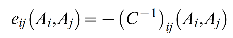
of the pair excess matrix restricted to (q−1) states (1≤Ai,Bj≤q−1) and
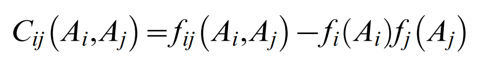
which contains the residue counts ƒij(Ai,Aj) for pairs and ƒi(Ai) for singlets in the multiple sequence alignment The parameters hi(Ai) are computed from single residue compatibility conditions. Given the formulation of the probability model (Equation 1), the effective pair probabilities are
These pair probabilities refer to the full specification of particular residues Ai, Aj at positions i and j. For the quantification of effective correlation between two sequence positions i and j, one has to sum over all particular residue pairs Ai,Aj to arrive at a single number that assesses the extent of co-evolution for a pair of positions. In analogy to mutual information,
such that the DCA coupling terms between columns i and j are given by
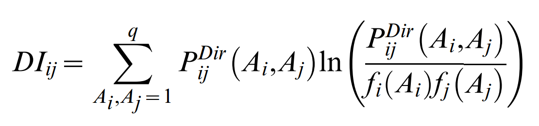
As there are L2 values DIij, and one expects residue contacts of the order of magnitude of L, only a relatively small number top-ranked DIij values (ordered in decreasing order of numerical value) are useful predictors of residue contacts in the folded protein. Given the analogy to statistical physics, the residue couplings eij(Ai,Aj), on which the DIij are based, can be thought of as pair interaction energies.
PSICOV Precise structural contact prediction using sparse inverse covariance matrix [3]
Note: this server uses FreeContact, an open-source EVfold-mfDCA implementation [4].
Inferring directly coupled sites using covariance
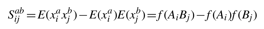
The starting point of our method is to consider an alignment with m columns and n rows, where each row represents a different homologous sequence and each column a set of equivalent amino acids across the evolutionary tree, with gaps considered as an additional amino acid type. We can compute a 21m by 21m sample covariance matrix as follows:
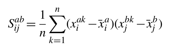
where xiak is a binary variable (x∈{0, 1}) indicating the presence or absence of amino acid type a at column i in row k and xjbk the equivalent variable for observing residue type b at column j in row k.
Based on the standard identity for covariance of Cov(X, Y)=E(XY)−E(X)E(Y), and the expectation of a binary variable E(x) being equivalent to the probability of a positive observation p(x=1), this simplifies to the following expression based on the observed marginal frequencies of amino acids (ƒ(Ai) and ƒ(Bj)) and amino acid pairs (ƒ(AiBj)) at the given sites in the set of aligned sequences:
Any individual element of this matrix gives the covariance of amino acid type a at position i with amino acid type b at position j. By calculating the matrix inverse of the covariance matrix, the precision or concentration matrix (Θ) is obtained, from which a matrix of partial correlation coefficients for all pairs of variables can be calculated as follows:
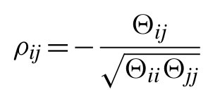
In the simplest case, a partial correlation coefficient can be calculated between two random variables with the controlling effect of a third random variable taken into account. The partial correlation matrix above, however, gives the correlations between all pairs of variables with the controlling effects of all other variables taken into account. Here, the partial correlation matrix gives the correlation between any pair of amino acids at any two sites, conditional on the frequencies of amino acids at all other sites. Thus, assuming the sample covariance matrix can in fact be inverted, the inverse covariance matrix provides information on the degree of direct coupling between pairs of sites in the given MSA. Off-diagonal elements of the inverse covariance matrix which are significantly different from zero are indicative of pairs of sites which have strong direct coupling (and are likely to be in direct physical contact in the native structure).
In general terms, where an inverse covariance estimate is constrained to be sparse, the non-zero terms tend to more accurately relate to correct positive correlations in the true inverse covariance matrix. The expectation of sparsity in this application is well justified from observations of contacts in known protein structures, where on average only around 3% of all residue pairs are observed to be in direct contact.
Sparse inverse covariance estimation
Let S be the empirical covariance matrix computed from a sequence of d-dimensional vectors, x1,…, xn, sampled from some fixed but unknown probability distribution. Matrix S can be computed as
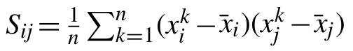
for every i,j=1,…, d, where x̄ is the empirical mean. The graphical Lasso is a statistical method which estimates the inverse covariance of the data by minimizing the objective function:
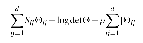
In this function, the d×d matrix Θ is required to be symmetric and positive definite. The first two terms in can be interpreted as the negative log-likelihood of the inverse covariance matrix Θ under the assumption that the data distribution is a multivariate Gaussian.
The third term is the ℓ1-norm of matrix Θ, a special kind of regularization or penalty term. One main insight behind such a regularizer is that it favours sparse solutions, in the sense that many of the components of the positive definite matrix Θ̂ which minimizes will be zero. The amount of sparsity in Θ̂ is controlled by the positive parameter ρ, which needs to be chosen by the user. Typically, as ρ increases the number of zero components of Θ̂ increases, eventually reaching the point where all the components are equal to zero.
The need for a sparse inverse covariance matrix is well understood when the data probability distribution is a multivariate Gaussian distribution with covariance ∑. In this case, it is well known that ∑−1ij=0 if and only if the variables i and j are conditionally independent. Hence, if we know a priori that many pairs of variables are conditionally independent, it seems appropriate to estimate the inverse covariance by the graphical Lasso method. The parameter ρ can be selected to reach a desired sparsity level, provided this is known a priori.
An important rationale for sparse estimation comes from the observation that in many practical applications the size of the matrix Θ is much larger than the number of data points n, but the underlying inverse covariance matrix which we wish to estimate is known to be sparse. Under this assumption and certain technical conditions, it has been shown that the solution Θ̂ of the above problem is a good estimate of the inverse covariance. More importantly, the sparsity pattern of Θ̂, namely the set of non-zero entries of this matrix, is close to the sparsity pattern of ∑−1, thereby providing a valuable tool for selecting the pairs of conditionally dependent variables.
We find the solution Θ̂ by solving the dual optimization problem and using the block coordinate descent technique. This formulation also allows one to use the more general penalty term ∑ijrij|Θij| where the rij's are some positive parameters, which incorporate prior knowledge on the relative important pairs of components.
A final point worth noting here is that while all of the above is under the assumption that input data distribution is multivariate Gaussian, it has been that this dual optimization solution also applies to binary data (as is the case in this application).
Shrinking the sample covariance matrix
Although the graphical Lasso approach works well in dealing with singular or poorly conditioned sample covariance matrices, the time taken to reach convergence can be problematic in some cases (e.g. families with few sequences or highly conserved regions). To speed up convergence, particularly in the worst cases, we condition the sample covariance matrix by shrinking towards a highly structured unbiased estimator:
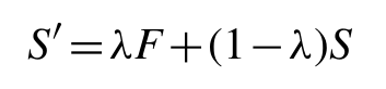
where F is the structured estimator matrix and λ is the so-called shrinkage parameter. The shrinkage target we used was F = diag(S̄,S̄,...,S̄) i.e. the identity matrix scaled by the mean sample variance (mean of the sample covariance matrix diagonal values).
Here, we use the simple ad hoc approach of gradually increasing λ until the adjusted covariance matrix is no longer singular i.e. has no remaining negative eigenvalues (tested by Cholesky decomposition). Given the large number of dimensions, this shrinking procedure is generally much faster than the more common approach of truncating negative eigenvalues after finding all the eigenvalues and eigenvectors of the matrix.
Having conditioned the covariance matrix by shrinking, the graphical Lasso algorithm is then used to compute its sparse inverse.
Final processing
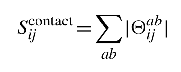
To arrive at the final predictions of contacting residues, for alignment columns i and j, the ℓ1-norm is calculated for the 20×20 submatrix of Θ corresponding to the 20×20 amino acid types ab observed in the two alignment columns (contributions from gaps are ignored):
To calculate a final score which has reduced entropic and phylogenetic bias, we can correct the raw precision norms Sijcontact using the same average product correction (APC) used to adjust MI for background effects. Thus, the final PSICOV score for positions i and j is given by:
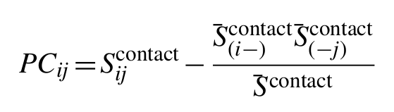
where S̄(i-)contact is the mean precision norm between alignment column i and all other columns, S̄(-j)contact is the equivalent for alignment column j, and S̄contact is the mean precision norm across the whole alignment. Finally, this background corrected score can easily be converted into an estimated positive predictive value by fitting a logistic function to the observed distribution of scores.
Sequence retrieval and MSA construction
The server working pipeline is as follow (see Figure 1):
Sequence retrieval
The inputs for the server are either two or more Uniport ID or protein sequences in one-letter-code format or FASTA format.
With each sequence a blast search is performed. Blast parameters are set at expected value = 0.001 and three iterations. Retrieved homologous sequences are filtered to save only one by NCBI Taxonmy ID (TaxID). If more than one sequence have the same taxID, we select the one with the lower e-value, If two or more sequences (with identical TaxID) have identical E-value, the one with the higher bit score is chosen.
In such a way we have a group of homologous sequences each one representing a unique TaxID.
Multiple Sequence Alignment
Alignment is performed with Mafft with the “auto” parameters setting. The user specified sequence or the first sequence (if the user uploaded an alignment) is set as the reference sequence. Alignments are trimmed by removing the positions with gaps in the reference sequence (gap-strip). Gaps in other sequences are allowed.
Multiprotein alignment construction
Aligned sequences of each group are paired up and concatenated if the two sequences have identical TaxID. In such a way we pair up sequences that are supposed to interact or at least, that the interaction is possible. The final MSA resembles a standard MSA but has the two sequences concatenated. This MSA is suitable for correlated mutation calculations. The only difference is that correlations between positions i and i+L (being L the lenght of the first protein) will be an interprotein positions correlation.
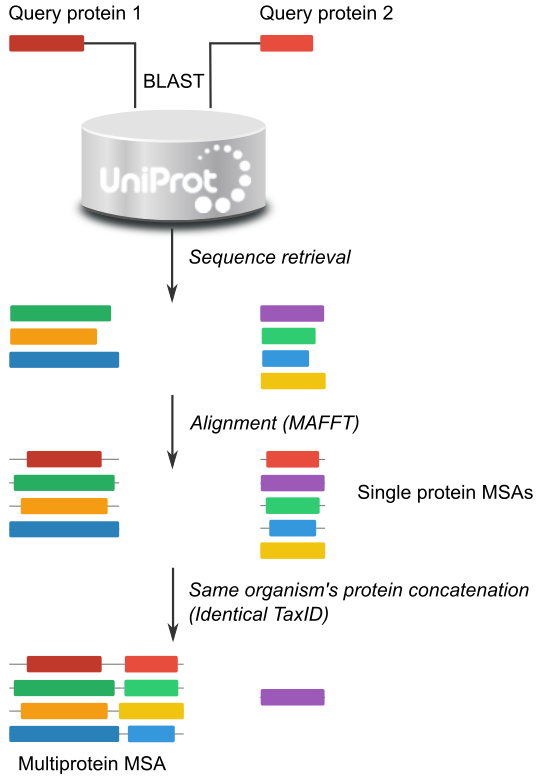
Figure 1: Schematic view of the workflow from the input sequence to the multiprotein MSA.
Upload you own alignments
The user can provide its own alignments. Note the the server will pair up proteins by the same position in the alignments (ej: protein 1 of family A with protein 1 of family B), no TaxID will be checked. It is mandatory that the user order the sequences in each alignment as if the corresponding sequence in the other alignment is the one it is supposed to interact with.
Inputs for running a job
The user can provide either the uniprotKB ID or protein sequences in one letter code of the sequences of interest.
Also, MSAs of the different proteins can be loaded. In such a case, proteins supposed to interact have to be in the same order in the alignments.
Server Results
Covariation Circos
Results are shown as a Circos representation for each proteins pair and each method (See Figure 2). In the outer circle the concatenated query sequences are shown in different colors, indicating the number and the amino acid residues of the reference sequence. The user can zoom in on any region of a graph to examine it more carefully.
The coloured square boxes of the second circle indicate the sequence conservation (highly conserved positions are in red, while less conserved ones are in blue). The conservation score was calculated as the information content, i.e: the maximum entropy whren the 20 amino acids are equiprobable, minus the Shannon entropy of the given position.
The inner circle represent the sequence positions in boxes colored in green or violet according to the sequence they belong to (protein 1 or protein 2).
The correlated mutation scores are represented as lines between positions in the center of the circles. Intraprotein relationships are coloured as the protein they belong to and interprotein correlations are coloured in red. In Figure 2 the MI score was used, but identical output will be displayed with DCA and PSICOV scores in the inner part of the circles.
The user can observe intra-protein, inter-protein or both inter- and intra-protein (Figure 2) covariation scores for one, two or the three methods (more circos can be unfolded by the “add new circos panel” option).
For each method, Intra-, Inter-protein or both scores can be visualized by clicking the checkboxes.
The threshold value to display the scores can be interactively selected with the scrollbar shown below the circos.
To keep in mind the importance of the interprotein covariation score, the server informs the position in which those scores are in a sorted list of scores (where both inter and intra-protein scores are listed). On the other hand, it is possible to analyse only the inter-protein scores. In that case we anyway inform which is the position in a sorted list with all the scores to bear in mind the strongness of this value compared to intra-protein covariation values.
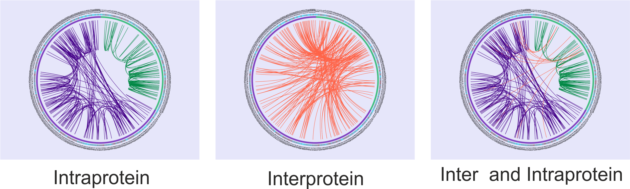
Figure 2: Circos displaying Intra-, Inter- and Inter- and Intra-protein MI score. Showing the first 200 scores.
Methods overlap
A visual inspection of the different results can be made by displaying one, two or the three circos in the results page (use the “add new circos panel” option).
On the other hand, the scores of the three methods can be downloaded to allow the user further analysis (e.g: Spearman rank correlation, EV-complex score calculation, etc).
The server also provides an option to calculate the circos with the overlapped results given a threshold for any two methods (Figure 3).
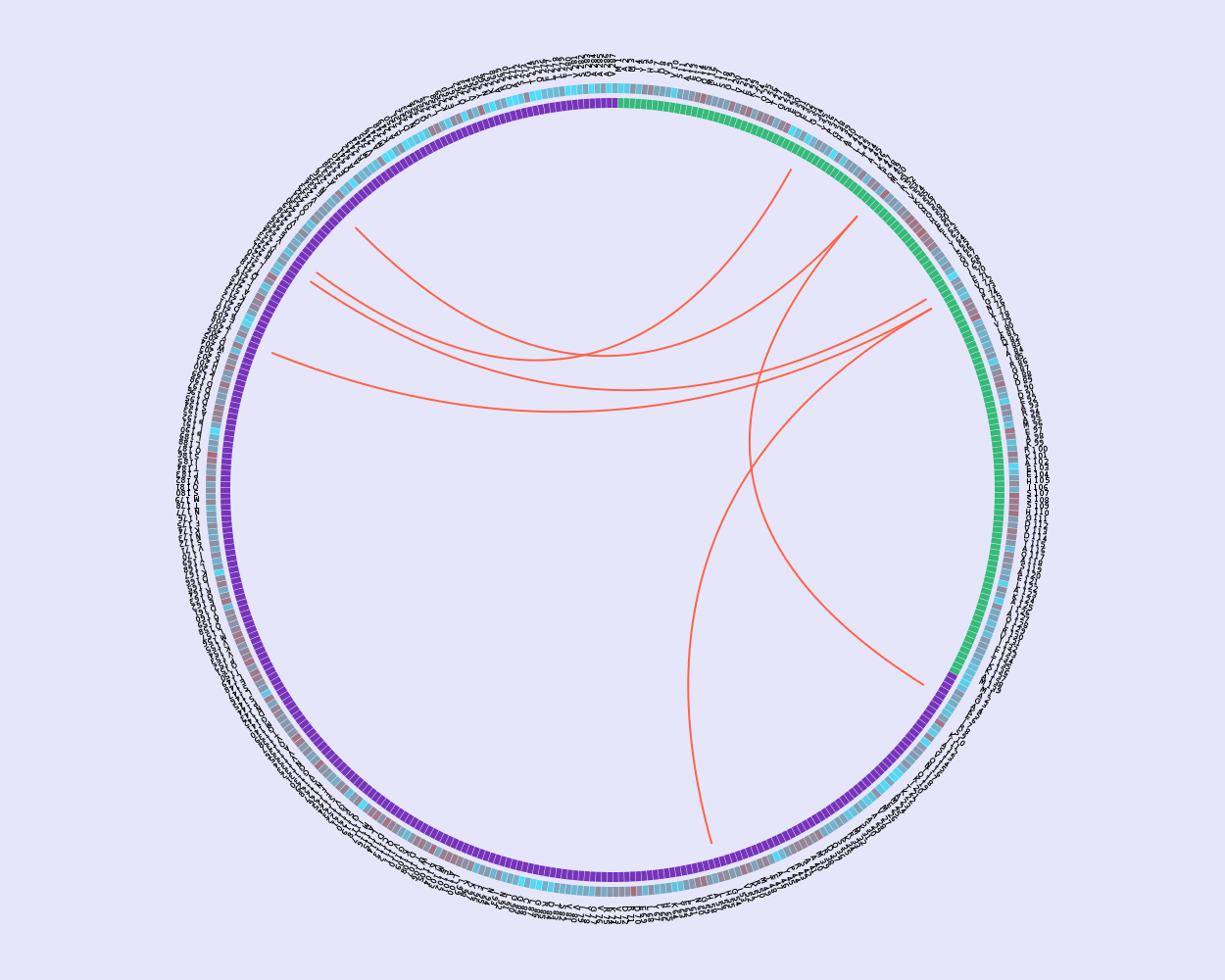
Figure 3: Circos of overlapped results. This circos representation shows overlapped results between the Top 200 scores of MI and DCA methods.
Covariation Matrix
The results of each method can be visualized in a matrix representation summarizing the top scores between all pairs of residues. This representation shows the Top 100, Top 500 and Top 2500 scores (Figure 4).
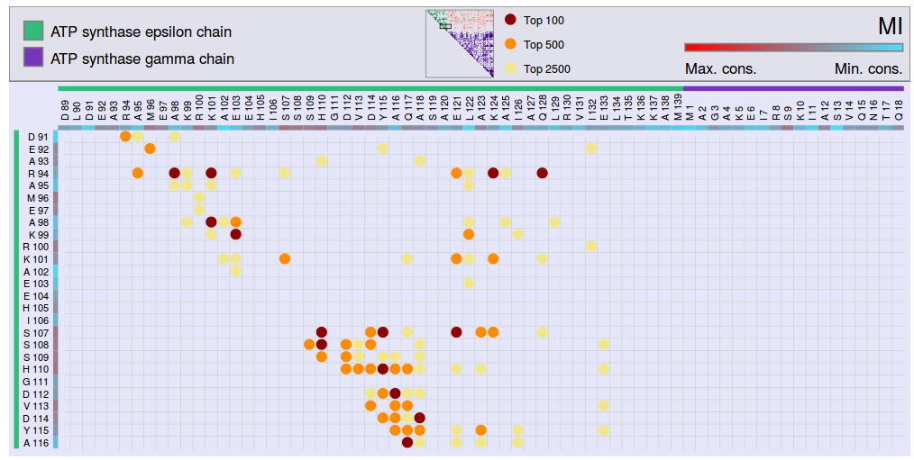
Figure 4: Covariation Matrix showing the Top 100 (red), Top 500 (orange) and Top 2500 (yellow) scores. This figure represents the MI score, but an analog matrix can be generated for each method.
References
-
Iserte JA, Simonetti FL, Zea DJ, Teppa E, Buslje CM.
I-COMS: Interprotein-COrrelated Mutations Server.
Nucleic Acids Res., vol. 43, issue. W1, pp. w320-325, Jul 2015. -
Buslje CM, Santos J, Delfino JM, Nielsen M.
Correction for phylogeny, small number of observations and data redundancy improves the identification of coevolving amino acid pairs using mutual information.
Bioinformatics (Oxford, England), vol. 25, no. 9, pp. 1125-31, May 2009. -
Marks DS, Colwell LJ, Sheridan R, Hopf TA, Pagnani A, Zecchina R, Sander C.
Protein 3D Structure Computed from Evolutionary Sequence Variation.
PLoS ONE 2011, 6:e28766. -
Jones DT, Buchan DWA, Cozzetto D, Pontil M
PSICOV: precise structural contact prediction using sparse inverse covariance estimation on large multiple sequence alignments.
Bioinformatics 2012, 28:184-190. -
Kajan L, Hopf T, Kalas M, Marks D, Rost B
FreeContact: fast and free software for protein contact prediction from residue co-evolution.
BMC Bioinformatics 2014, 15:85.